

How to stay sane with your personal finances in South East Asia
When I moved to South East Asia, I knew that money will work a little differently. Coming from Germany I'm used to cash.
When I moved to South East Asia, I knew that money will work a little different. Coming from Germany I'm used to cash. We have a saying: "Nur Bares ist Wahres" meaning "Cash is King". Wanna pay for your coffee with your card? Good luck
This might come as a surprise to other people from Europe. Having lived in the Netherlands for 1 year, I got so used to paying with my card everywhere, that when I came back to Germany for the first time after a while, I didn't understand why they wouldn't let me pay for my coffee with my card. Minimum spend 10€. eWallet? What's that? People usually use only 1-2 cards and of course cash.
Now I'm living in Malaysia. I have HSBC, BigPay, Fave, Boost, TouchNGo and Grab. I'm also using TransferWise. So I have 7 different ways to pay, always choosing what is the most convenient at any given moment. Also, I daisy chain my wallets together. Fave I pay with Boost, Boost I top up with BigPay and BigPay I top up with my HSBC account. This allows me to maximize perks such as AirAsia Big Points that I accumulate.
However, there's a price to pay for that, which is visibility over your personal finances. Financial literacy is a big challenge (with only 24% of Millenials having a good overview of their personal finances). I recently went through Lifebook, an exercise that gives you clarity over all areas of your life and how to improve them. One big area of improvement for me is financial. No matter how much salary I earn, I will always end up with a zero in my bank account by the end of the month. I wanted to get a grip on my financials; make a monthly budget and track it.
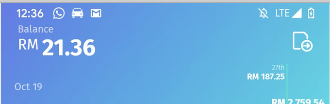
That's why I was so excited about BigPay's analytics feature. I told myself I will only use BigPay from now on so everything will be consolidated in one account and I know exactly what I spend my money on.
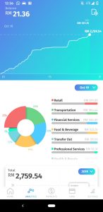
Looks good enough, at first glance... What the hell are financial services and why do I spend 20% of my overall monthly spendings on it?

While BigPay is smart enough to categorize Fave payments into Wellness or Food & Beverages based on the merchant I paid at, the fact that I am using Boost to pay for Fave and BigPay to top up Boost, basically most of my daily spendings go into Financial Services. And when I order food with Grab, it ends up in Transportation. Don't get me wrong. I love BigPay and their financial analytics feature is very solid, but it just doesn't work enough for me. I wanted a better solution:

Cue In: My own financial analytics tool powered by Google Spreadsheets. It pulls in data from all my various payment methods, organizes them, tags automatically based on previous payments where it can and lets you tag the remaining transactions on your own.
There were some problems I needed to overcome and I will run you through on how I solved them, so you can build your own tool. It took me around 6 hours to build it. Following this guide, I guess you will be able to do it in 30 minutes!
Don't want to go through the trouble of building it on your own? Contact me to get it directly.
Please note that I obscured my data in the examples below. If you want to know my finances, ask me personally 😝
1. Data organization:
Google Spreadsheets has a limit of cells that can be used in one file. Also, it is notorious to get overwhelmed if there are too many calculations in one sheet. So I knew I had to create one main sheet as a final analytics tool where everything comes together and that is fed the crunched and organized information from somewhere else. Additionally, I chose to create individual sheets for the financial data for each of the months. I reckoned this to be the swiftest way to plug in the upcoming months.
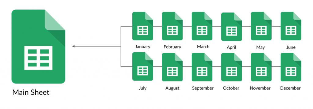
We'll start by creating one sheet for the first month.
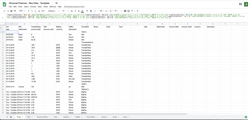
Within the sheet Personal Finances - Raw Data - Template, I then created one tab for each financial service that I wanted to plug-in, as well as one tab that would create one final list of all my transactions across all services.
2. Gathering the data
The next step is to basically download a list of transactions from each of the services. You would think this is the most straight forward. Every service should have some sort of export service, right? Well... most of them do. As you will probably use different financial services than me, they will each work a little bit differently. I am showing you the examples I used, which will help you figure out how to do it for yours.
ING
The first on the list was pretty straight forward. Log in to Mijn ING and press the Download icon for the account you want the transaction list from. It will ask you to put in the date-range as well as choose a download type. Choose CSV! Then you simply copy and paste it into the respective tab you created in your Google Sheet

TransferWise

Similarly, straight forward, you go to the balances of your Borderless account, select a balance and press the download statement link and make sure to choose CSV. TransferWise right now does not allow you to download one list for all of your balances, but you need to download the CSV for each balance. Since their structure is always the same, you can simply paste them in the same tab one after another. Just make sure to remove their headers.

N26
N26 also knows the value of providing an easy-to-access CSV download and parks it right in front of you when you login and land on the front-page:
Simply choose the time-frame and download the CSV and copy and paste it into your Google Spreadsheet.
BigPay
There's no website that you can log in, but on the app on the Analytics screen is a button on the top right that lets you choose the month you want to export and allows you to share an Excel file. Just send it to your email address and download it. If you don't have Excel, upload it to Google Drive and convert it.
HSBC
Even though HSBC does not offer a CSV export feature, it is still very easy to get your transaction list. HSBC displays all your transactions in a simple table that you can actually just copy and paste directly into your Google Spreadsheet.
TouchNGo
Just like BigPay, for TouchNGo you access the Transaction History from the app. You can find the button on the main screen. Select the timeframe and email the CSV file to you.
Boost
There's, unfortunately, no way for you to download the transaction list by yourself. I thought I'd give it a shot and send a request to their support team, and actually, within 24 hours, they did send me my full transaction list. Just make sure to tell them the time-frame you want. They give it to you in an easily copyable table.
Grab
There's a website that you can access from your computer browser where you log in, verify your login with your Grab app and then easily download your transaction details as CSV.
Fave
For Fave, you simply login and navigate to your Payment History. Copy and paste the table into your Google Spreadsheet and you're set.
3. Linking the data
Now we have all the data in one file. However, right now they're all in separate tabs. In order to easily access and analyze them, we need them in one list. We're going to want to get the information about the date, whether it was debit/credit, the debit amount, the credit amount, currency, a description as well as the financial service. For each of the payment services, the transaction list is structured differently. This is where we utilize one of the most powerful functions in a Google spreadsheet. The query function.
Let's break it down.
The overall function is encompassed by curly brackets { }. This means that whatever is within the curly brackets, separated by ; will be returned in one table. This is basically what fuses all the tabs together in one list of transactions. Then we have one query function for each of our financial sources. I will explain the structure on the basis of the BigPay example, which should make it clear for the rest of them.
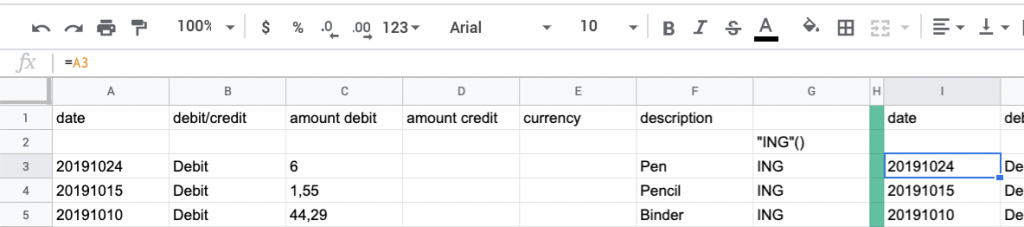
The query function is receiving two parameters. The first parameter is the data source for where the function will get its information from. We're using indirect, because we are dynamically getting the name of the sheet from the cell E1. If you check the screenshot above, you will see that the value of that cell is BigPay. Without a dynamic reference in the query, the parameter would simply be "BigPay'A$2:Z$1000". We're using & to fuse together the different parts to build the parameter. The second parameter is the actual query. If you're familiar with SQL, you will feel at home here. Since in Parameter 1, we specified that we're selecting data across column A to Z, we can reference each of these columns and you can even specify the order in which you want them to be returned. In this example, we are selecting the columns B,Z,F,Y,G,D and we're putting them in this specific order, so it will fit into the order of date, debit/credit, debit amount, credit amount, currency, description.
date is in column B. BigPay does not give us a differentiator between debit/credit, so we need to leave it empty, and we do so by selecting column Z (which is empty). debit amount is in column F. There is no credit amount, so again, we need to leave it empty and choose column Y. currency is column G and description is column D. But what about the column for financial service?
Let's take another close look at our query: "select B,Z,F,Y,G,D,'BigPay' WHERE B is not null" . You will see that we are specifying 'BigPay' as if it were a column. This leads to us adding one more column for the financial service to our main transaction list. Lastly, we are utilizing a WHERE parameter that filters out any row where column B (date) is not empty. The reason for this is that in our parameter 1 we are referencing all cells from A$2:Z$1000. This would import hundreds of empty rows into our main transaction list. We don't want empty rows there.
You can follow the same logic to plug-in transaction lists from any other financial service.
4. Importing the data into the main sheet
Since we now have the full transaction list done for one month, we want to import it into our main sheet. This is very straight forward. Google Spreadsheet offers the simple IMPORTRANGE function. Super powerful if you know it's limitations: once imported, you cannot sort or filter it. You also cannot make any changes. Try doing it and see what happens. I'm serious. Go ahead. Try it. What you will have seen is that it simply does not accept your changes. Either it stays the same as it is, or it breaks. This is because while usually in Excel or Google Sheets, you will have a specific value assigned to each specific cell, the IMPORTRANGE function simply tells Google Sheets: from cell A1 on fill up whatever you are taking from the source sheet. The cells that are being filled do not actually hold any value.
Let's first create our tab. In this example, we will call it Oct Raw. In A1 we use the IMPORTRANGE function, which needs 2 parameters. The first parameter is simply the link to your other spreadsheet and the second parameter is the range that you want to import. In the range, you need to specify not only the cell range but also the name of the tab. So if you called the main transaction list Total, the final function will be:
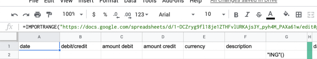
You will see that we imported date, debit/credit, debit amount, credit amount, currency, description, financial service into columns A to G. Now to overcome the limitations of the IMPORTRANGE function, we will simply work in the columns I to N to correct our data and build a new table. In the new table, we will make sure that every cell actually holds the correct value, allowing us to sort, filter and do all sorts of fun things.
5. Correcting the data
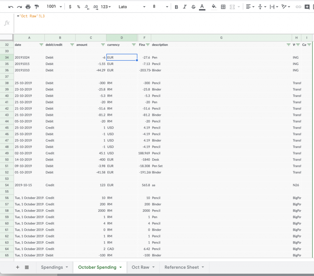
You will probably have noticed a big challenge by now. Even though we were able to create one full transaction list including all financial services, there's a lot of discrepancies.
Problem #1: Transferwise denotes debit with a negative value while BigPay denotes it with a positive value.
Problem #2: Some transactions are in MYR, some in SG and some in EUR or CAD.
Problem #3: HSBC has a column for credit and one for debit. Values are always positive.
Problem #4: ING uses the same column for debit and credit. Values are always positive, but it will denote a transaction as debit or credit in the debit/credit column.
Problem #5: HSBC is introducing a comma for 4 digit numbers.
Problem #6: Fave is separating decimals with a comma instead of a period.
So how do we clean up this mess?
The easiest way for us to deal with this is to properly predict whether a transaction is credit or debit and normalize them in a way for us to easily read them. In the best way, we want to be able to put all transactions in one list, credit as positive numbers and debit as negative. This will allow us to easily summarize our balance later. So how do we do this?
Let's start with the easiest: date. This is pretty simple:
Next up is debit/credit. We will create a formula that will predict with 100% accuracy if a row is a debit or a credit transaction.

Let's break it down:
The IF function takes three parameters. The condition, what happens if the condition is true and what happens if the condition is false. As you can see, this is just a chain of IF conditions. Let's go through it line by line:
Line 1: If A3 (date) is empty, it means there is nothing, so we display nothing (denoted as ""). If it is not empty, then:
Line 2: ING is so nice to denote a debit transaction as debit, so we can just take this.
Line 3: Checks if D3 is empty. len(D3) will calculate the number of characters and if they're more than 0, we know there's a value in the credit column and it automatically makes it a credit transaction. This is the HSBC case.
Line 4: Now we're checking for Transferwise and BigPay as they're cases are quite similar. That's why we have the last column.
Line 5: We are using the search function to look for the character -. If the search fails and returns an error, we know that it has to be a Credit transaction, as TransferWise and BigPay put a - before the transaction amount of debit transactions. Please note that we have to do this because Google Sheets does not know we're dealing with numbers. It thinks this is text. We could tell Google Sheets that we're dealing with numbers, which would then require a. different logic.
Line 6: Now we're checking for the N26 case, which is so nice to tell us that a transaction is Income.
Line 7: Whereas TouchNGo denotes debit transactions as Payment.
Line 8: For HSBC, we know it's a debit transaction if D3 is empty.
Line 9: Which leaves us with Grab and Fave, which do not record any credit transactions and are debit by default.
Whenever you're adding a new financial service, you will have to rework that logic to work for you. It is essential for the next step, which is to build one clean list of all transactions that we can then just summarize over.
amount:

Let's break it down
The logic of that formula is that if column J is Debit, the value for amount will always be negative. So let's take it bit by bit and let's start with this part (line 2-3)
You will see that the result for when J3="Debit" is true is almost the same as when it is false, just that we multiply it by -1. The function abs(VALUE(SUBSTITUTE(split(C3,"RM") , "," , "."))) converts any value in a positive number. abs gives you the absolute of any value, meaning if it's a negative value, it becomes positive and positive stays positive. VALUE converts text into a number, so that the abs function will recognize it. split(C3,"RM") ensures we account for the case of TouchNGo where it will keep the currency in the amount. We are basically removing the two letters RM. Lastly, the SUBSTITUTE function removes any comma and replaces it with a period. This is for the case of Fave.
For the case of HSBC, C3 will be empty and this function will throw an error. Hence this part is wrapped in an IFERROR function, which throws the following in case of error (line 6-7):
As you can see this function uses D3 instead of C3, getting the value from column D (credit). One difference is that HSBC introduces a comma separator for the thousands, leading to an error. Thus, there's an additional IFERROR function, which will simply remove the RM denotation and converts it directly to a number.
Finally in the case of HSBC and the transaction being debit with the amount being denoted in the column C, the function results in an error and will trigger the final piece:
Finally, if all functions trigger an error, we will return a 0. This is for the case of Fave, where failed transactions are still displayed with an empty cell in Column D.
Next up is currency.
=IF(A3="","",IF(OR(G3="ING",G3="N26"),"EUR",IF(OR(G3="HSBC",G3="TouchNGo"),"RM",IF(E3="MYR","RM",E3))))
We're simply checking for each financial service and making sure the currency denotation is uniform.
description and Wallet can simply be referenced from the original table and with this we're almost done.
6. Category annotation tool
Now we have a fully automatized tool to normalize our different transactions. Good job! However, this will still not give us visibility over our personal finances. We need to be able to annotate the categories - and in the best case, it should be. automatic.
Google Sheets cannot do magic, so in any case, the annotation will have to be based on previous data and we do not have previous data. So for now, we will annotate manually. We will do this in a new tab, which we will create for this. The reason is that we want to format our transaction list to make it more easily readable, i.e. expand the description column, etc...
We are simply referencing back to Oct Raw. We are not copy and pasting. So for A1 you put =I1, B1=J1, D35=L35 and so on. You do this by filling it for A1, copying A1 and pasting it over the entire sheet. Then you add a column I and start entering which financial category each transaction belongs to. You should think before how specific you want to track and for which categories you want to put yourself a budget. Then you fill that column completely for every transaction.
Note: One issue I found was that I was not sure what to do with transactions i.e. when I would pay with Fave and this could trigger 2 transactions: a debit transaction under Fave for paying the merchant and a credit transaction under Boost, paying for Fave. In this case, I would only categorize the Fave transaction. The Boost transaction, I would simply denote as "Money transfer". Same principle would be applied when I transfer money from HSBC to BigPay. Both the debit on HSBC and the credit on BigPay would simply be denoted as "Money transfer".

Once filled, you copy the columns G, H, J (description, Wallet, Category) and into a sheet called Reference Sheet. Make sure you only paste the values. You can use right click -> Paste special -> Paste values only for that.

After that, we will want to filter out all duplicates from column A (description) by putting this function in C2: =unique(A3:A). From this list of unique descriptions, you will match the respective category. You do this with the VLOOKUP function:

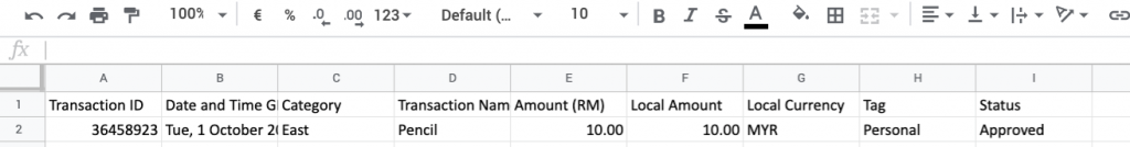
The VLOOKUP function will check for the value in D2 if it can find it anywhere in the range of A:C. If it finds it, it will take the value from the 3rd cell of the row it found the value... I know this was a quote complicated sentence.
So let's explain it using the picture above: The result of the function =vlookup(D2,A:C,3,false) is Banking Fees. This result gets produced as the function is looking for the value Pencil in the columns A, B, C. It will find Pencil in row 3. As Pencil is in column A, it is the 1st cell. In the 2nd cell it says ING and in the 3rd cell it says Banking Fees. Since we told the function to look in the 3rd cell, it will return that value.
You copy that function over the entire column E to finish your final unique references.
Note: Now whenever you finished adding a new month, all you need to do is to copy and paste the columns description, Wallet, Category from your Spending sheet to the end of this sheet to expand the knowledge of your Automatic Reference sheet.
Now we basically trained the. Automatic Reference sheet with your category annotation. To demonstrate the power, we will use it to re-predict the categories for the transactions we have just filled. I know this is a silly exercise, but by doing this, we will finish the template that you can simply re-use when you want to create the Spending sheet for the next month, in which case it will actually be able to predict the category for some of your transactions.

The function we'll be using is also the VLOOKUP function. This time we use it to search across two different sheets. It will try to find the description in the list of unique descriptions matched to categories in the Reference Sheet that we have just created. If it does not find anything, it will display nothing, which means you will have to fill the category by yourself.
7. Adjusting currencies
If you paid attention, you will notice that we actually never took action on the currency. If I have spendings in EUR and in RM, I need to adjust for currency conversions. We could've done this in the very beginning in our Raw sheet, however, I chose to build this tool to give the flexibility to adjust for currency conversion on a monthly basis.
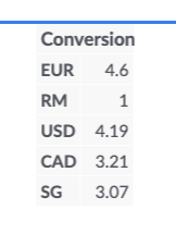
You need to choose one currency in which you want to build your final summary. I chose to track my spendings in RM, which is why it is denoted as 1 as the baseline. Then you simply google the currency conversion. I.e. EUR4.6 = RM1.

=IFERROR(vlookup(D34,H$5:I$9,2,false)*C34,"")
You add an additional column next to currency and use the VLOOKUP function again to be able to find the corresponding currency conversion value to the designated currency (D34) in your Conversion Table (which is in my case in H$5:I$9). Then you multiply it by the amount (C34). Simply copy and paste this formula over your new column.
Note: You probably know this but when you copy formulas, Google Sheets will automatically adjust the cell references for you. I.e. you reference cell C4 in a function, you copy and paste it to the cell to its left, it will be B4, whereas if you posted it to the cell one below, it would become C5. If you put $ in front of the letters or the numbers, they will not be adjusted automatically, which is what we want in this case.
8. Summarizing the spendings
Now we have a fully categorized list of transactions and the ability to predict the category of our future spendings automatically. We're fully set with an automatic workflow to replicate these steps for the next months in a matter of minutes. What we're missing, however, is to properly display our spendings per category.

You can go ahead and design it however you want. What is important is that you'll want a list of all the categories that you've used to categorize your transactions. Next to it. you can put your monthly budget and then we will calculate how much you actually spent for each category.

=sumif(I$26:I,B5,F$26:F)
The SUMIF function will sum up all values in a column if one condition applies. The first parameter I$26:I is the range it will sum up. It will check for each of the values if the value in the column F (from the third parameter) will be the value in the respective cell B5. By using $ we can just drag it down the column to get the sum for all your categories.
That's it! You're done. Congratulations. I hope you enjoyed it.
Let me know if you have any feedback to the sheet. I would love if you share any improvements and suggestions you have to this tool.
Got inspired by what is possible with simple, freely available tools and require a solution for yourself? Get in touch with me!
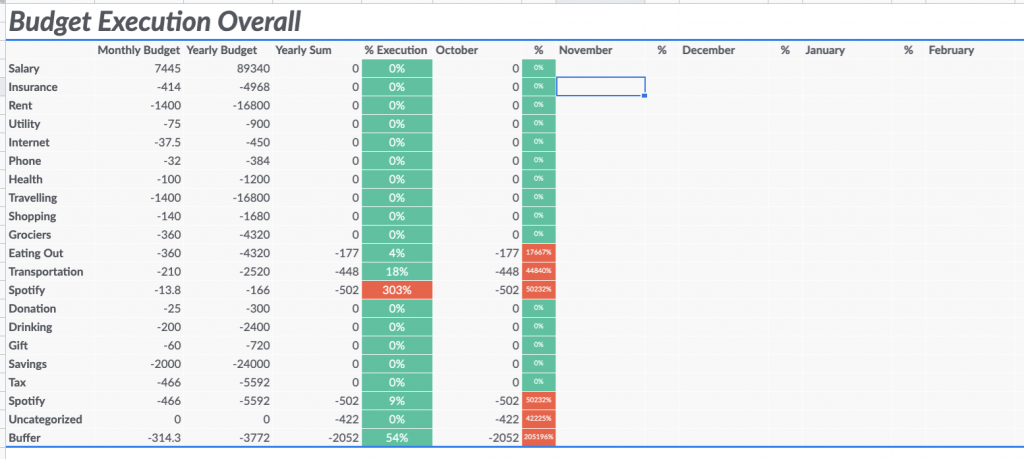
By the way: this is not everything. I've also worked on a yearly overview and breakdown that will be updated automatically.
How to stay sane with your personal finances in Southeast Asia was originally published in Laurins Page on Medium, where people are continuing the conversation by highlighting and responding to this story.
.jpg)

